Back to Seapacer Home Page

Background

The fuel costs are the second largest item (after salaries) on a big ship's budget. The fuel consumption for a large ferry ranges  between 1000 and 5000 liters per hour. This means that the ship consumes more oil per hour than a one-family house does for one whole year's heating (in northern Sweden). The price for the high quality bunker oil common in use is about 140$ /1000 liters (1994). The annual fuel budget for a ferry running 20 hours per day is consequently in the order of 2.5 million dollars. A reduction of 1% off the fuel consumption means an annual saving of more than 25.000$. The route planning of a ship with varying speed in different parts of the route aims at keeping the set arrival time while reducing the total fuel consumption.

What Affects the Fuel Consumption

Following are some of the most important factors:

	Ship specific parameters such as form of the hull, weight, type of main engines, propellers, etc.
	Number of engaged main engines.
	The ship speed relative to ground measured in knots (denoted "bottom track speed").
	Water currents (direction and speed in knots).
	Water depth.
	The ship's draft (depends on the cargo).
	Wind (direction and strength measured in Beaufort points).

How Can the Fuel Consumption Be Reduced ?

The method we are considering here is called "route planning." It consists of the ship's varying speeds in different parts of a route. Since the external conditions (wind, current, and depth) vary, it is evident that fuel consumption cannot be maintained at a minimum if a constant speed is being kept throughout the route. Therefore, we get a minimization problem that has to be solved numerically: we have to find the speed distribution that minimizes the total fuel consumption, within the constraint of keeping the scheduled arrival time. Route planning of some kind or another is done on all ships. Most often the "calculation" consists of manual estimates based on previous experience from the same route.

SeaPacer

Seapacer is a control computer used on cargo ships and ferries to save fuel, primarily by automatic route planning. Wind, current, and water depth can be input by the operator before departure or during the voyage. Seapacer then automatically calculates a speed profile that minimizes the total fuel consumption. Based on the computed speed profile, Seapacer regulates the ship's speed by controlling the main engines and the propellers. The arrival time is kept without unnecessary margins and fuel saving of 5-15% is achieved.

The following is a description of the basic route planning system of Seapacer.

Models

The dependency of fuel consumption upon speed, wind, and water depth has been examined for many ship types. No mathematical relations have been found, only the sampled values. The following values have been collected on a ferry running between Hook van Holland and Harwich on the English Channel. Evidently, the sampled values do vary from ship to ship but they normally share the same characteristics.

Speed Models  F(xw)

The figures in the following table have been collected (with no influence from limiting water depth). They show fuel consumption for different speeds (in knots):

Table 1:

Speed through water  (xw)	Liters/hour
10.4	650
13.2	875
17	1300
20.1	2120
20.7	2900

Depth Model D(x, d)

At limiting water depths the ship's speed decreases due to the increased water resistance. In very shallow waters (a few meters below the keel), the so-called "squat effect" pulls the ship downwards, thereby further reducing its speed. The following table shows the effect of water depth on fuel consumption at varying speeds and water depths:

Table 2

Speed over Ground (x)	Depth (d)	Increased Fuel Consumption %
10.0	8	5
10.0	10	3
10	100	0
17.0	8	20
17.0	15	10
17.0	100	0
23	8	30
23	15	20
23	100	0

Values in between these points are estimated by a 2-dimensional linear interpolation.

Wind Model W(w, wd)

The wind is specified by the direction relative to the ship's course and the wind strength expressed in Beaufort points. The parameter wd is the wind direction (degrees). w is the Beaufort degree (0-10).

Generally speaking, wind from the side and even slightly from behind increases the fuel consumption due to the large open surface on the sides of many ships. The following table describes a typical and approximate relation between increased wind strength, direction, and increased fuel consumption:

Table 3:

Direction (wd)	Type	Increased fuel consumption % (for each Beaufort)
315-360, 0-45	Head wind	4.0
45-135, 225-315	Side wind	2.0
135-225	Tail wind	1.0

Values in between these points are estimated by a linear interpolation.

Example:

The ship is running at 18 knots. The current is 1 knot along the direction of the ship. The wind blows 4 Beaufort points straight against the starboard side of the ship (wd=90).

The water depth is 15 meters below the keel.

The speed through water is then 18-1=17 knots.

Table 1 shows the fuel consumption, before the wind and limited depth effects have been taken into account, at 1300 liters/hour.

Table 2 shows the fuel consumption increase by 10%, caused by the water depth.

Table 3 gives  4 * 2% = 8% increase due to the side wind.

The total fuel consumption in the example is therefore

1300 * 1,10 * 1,08 = 1544 liters/hour.

Formulating the Optimization Problem

The route is divided into n parts, each having constant depth, wind, and current conditions.

n is typically between 2 and 40.

Each part is denoted "route leg" or just "leg".

For each leg i, the following data is available:

	Length si (nautical miles)
	Longitudinal current component cli , (unit: knots) parallel to the ship's direction
	Transversal current component cti , (unit: knots) perpendicular to the ship's direction
	Wind strength wi(Beaufort)
	Relative wind direction wdi . (0.-360) (see Table 3)
	Water depth di (meter) below keel
	Minimum allowed speed xmini (knots).
	Maximum allowed speed xmaxi (knots)

For the route as a whole, the following data is provided:

	Total travel time T (unit: hours)
	Number of legs in the route

The ship's speed relative to ground is given in knots. 1 knot equals 1 nautical mile per hour.

The speed relative to ground x, is related to the speed through water (xw) and the current components ctand cl according to:

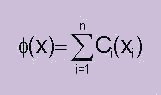
In other words: addition of the speed and current vectors

The fuel consumption (liters) on a leg i is denoted C_i and is a function of speed over ground x_i and the properties of leg i ; the length s_i , the current cl_i , ct_i , the wind strength w_i , the wind direction wd_i and the water depth d_i:

C_i ( x_i ) = s_i / x_i * F( xw_i ) * ( 1 + D(x_i , d_i )/100 ) * ( 1 + W( w_i , wd_i )/100 )

where F, D and W are given by table 1, 2 and 3 respectively.

The factor s_i / x_i is the time (hours) that the ship is on route leg  i.

x is defined as ( x₁ , x₂ ,..., x_n ),  i.e. the unknown speeds (over ground) on the n legs.

The total fuel consumption ffor a voyage is given by:

Constraints

As constraints we have:

1)

i.e. the ship has to arrive on time

and

2)

xmin_i £ x_i £ xmax_i , " i

These constraints can be used to define speed limits on parts of the route and also to set the available speed register for the ship.

f (x ) should now be minimized with respect to x under the above mentioned constraints.

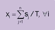
Start value algorithms

As start value, at least three methods are possible:

1)

Assign an equal speed to all legs. I.e:

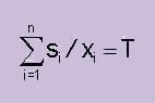
This method hardly needs any calculations, but on the other hand does not take either current, wind or water depth into account.

2)

Compute one value for speed through water (xw) on all legs that make the ship arrive on time (i.e. fulfills constraint 1 above).

This means that legs with counter current are run at a lower speed through water than legs with current along.

Compute a xw that solves:

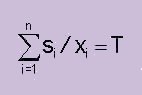
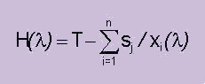
If constraint 2 states that x_i is not a valid speed over ground on leg i, assign one of the end points in the constraint to x_i.

This method gives an x vector that compensates for current but not for water depth or wind.

3)

Choose the fuel consumption (liters/hour) that, if used on all legs on the route, makes the ship arrive on time (fulfills constraint 1 above). This means that legs with counter current are run at a lower speed over ground than legs where the ship runs with the current. It also means that legs with heavy load due to shallow water and wind are run slower than other legs. This is intuitively correct and gives a very satisfactory result in practical tests.

The algorithm is two nested equations:

Find the fuel consumption (liters/hour)lthat solves H(l ) = 0 where H(l ) is defined as:

where x_i(l)is the speed achieved on leg iwith the fuel consumption lliters/hour.

x_i(l ) is consequently the x_i that satisfies:

( C_i(x_i) * x_i/s_i ) - l = 0

If constraint 2 above states that x_i is not a valid speed over ground on leg i, assign one of the end points in the constraint tox_i.

This method gives an x vector that is most often very close to the optimum and can be used to select the speeds on the different legs on the ships route.

The optimization is repeated at certain interval and also when new data for current, wind or depth is input during the voyage.